MAG generation
Generation of metagenome assembled genomes (MAGs) from assemblies
Assessment of quality (MIMAGs)
Taxonomic assignment
Prerequisites
For this tutorial you will need to first start the docker container by running:
sudo docker run --rm -it -v /home/training/Binning:/opt/data microbiomeinformatics/mgnify-ebi-2020-binning
password: training
Generating metagenome assembled genomes
 Learning Objectives - in the following exercises you will
learn how to bin an assembly, assess the quality of this assembly with
checkM and then visualise a placement of these genomes within a
reference tree.
Learning Objectives - in the following exercises you will
learn how to bin an assembly, assess the quality of this assembly with
checkM and then visualise a placement of these genomes within a
reference tree.
As with the assembly process, there are many software tools available for
binning metagenome assemblies. Examples include, but are not limited to:
MaxBin: https://sourceforge.net/projects/maxbin/
CONCOCT: https://github.com/BinPro/CONCOCT
COCACOLA: https://github.com/younglululu/COCACOLA
MetaBAT: https://bitbucket.org/berkeleylab/metabat
There is no clear winner between these tools, so the best is to experiment and compare a few different ones to determine which works best for your dataset. For this exercise we will be using MetaBAT (specifically, MetaBAT2). The way in which MetaBAT bins contigs together is summarised in Figure 1.
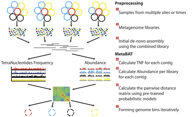
Figure 1. MetaBAT workflow (Kang, et al. PeerJ 2015).
Preparing to run MetaBAT
Prior to running MetaBAT, we need to generate coverage
statistics by mapping reads to the contigs. To do this, we can use bwa
(http://bio-bwa.sourceforge.net/) and then the samtools software
(http://www.htslib.org) to reformat the
output. This can take some time, so we have run it in advance.
 Let’s browse the files that we have prepared:
cd /opt/data/assemblies/
ls
You should find the following files in this directory:
contigs.fasta: a file containing the primary metagenome assembly produced by metaSPAdes (contigs that haven’t been binned)
input.fastq.sam.bam: a pre-generated file that contains reads mapped back to contigs
To generate the input.fastq.sam.bam file yourself, you would run the following commands:
cd /opt/data/assemblies/

# if you would like to practice this now, back up the input.fastq.sam.bam file that we provided first,
# as these steps will take a while:
mv input.fastq.sam.bam input.fastq.sam.bam.bak

# NOTE: you will not be able to run subsequent steps before this workflow is completed because you need
# the input.fastq.sam.bam file to calculate contig depth in the next step

# index the contigs file that was produced by metaSPAdes:
bwa index contigs.fasta

# fetch the reads from ENA
wget ftp://ftp.sra.ebi.ac.uk/vol1/fastq/ERR011/ERR011322/ERR011322_1.fastq.gz
wget ftp://ftp.sra.ebi.ac.uk/vol1/fastq/ERR011/ERR011322/ERR011322_2.fastq.gz

# map the original reads to the contigs:
bwa mem contigs.fasta ERR011322_1.fastq ERR011322_2.fastq > input.fastq.sam

# reformat the file with samtools:
samtools view -Sbu input.fastq.sam > junk
samtools sort junk input.fastq.sam.bam
Running MetaBAT
Create a subdirectory where files will be output:
cd /opt/data/assemblies/
mkdir contigs.fasta.metabat-bins2000
In this case, the directory might already be part of your VM, so do not worry if you get an error saying the directory already exists. You can move on to the next step.
Run the following command to produce a
contigs.fasta.depth.txt file, summarising the output depth for use with
MetaBAT:
jgi_summarize_bam_contig_depths --outputDepth contigs.fasta.depth.txt input.fastq.sam.bam
Now you can run MetaBAT as:
metabat2 --inFile contigs.fasta --outFile contigs.fasta.metabat-bins2000/bin --abdFile contigs.fasta.depth.txt --minContig 2000
We set the minimum contig size to 2000 using the --minContig parameter
Once the binning process is complete, each bin will be
grouped into a multi-fasta file with a name structure of
bin.[0-9].fa.
Inspect the output of the binning process.
ls contigs.fasta.metabat-bins2000/bin*
 How many bins did the process produce?
How many sequences are in each bin?
Obviously, not all bins will have the same level of accuracy since some might represent a very small fraction of a potential species present in your dataset. To further assess the quality of the bins we will use CheckM (https://github.com/Ecogenomics/CheckM/wiki).
Running CheckM
CheckM has its own reference database of single-copy
marker genes. Essentially, based on the proportion of these markers
detected in the bin, the number of copies of each and how different they
are, it will determine the level of completeness, contamination
and strain heterogeneity of the predicted genome.
Before we start, we need to configure checkM.
cd /opt/data
mkdir /opt/data/checkm_data
tar -xf checkm_data_2015_01_16.tar.gz -C /opt/data/checkm_data
checkm data setRoot /opt/data/checkm_data
This program has some handy tools not only for quality control, but also for taxonomic classification, assessing coverage, building a phylogenetic tree, etc. The most relevant ones for this exercise are wrapped into the lineage_wf workflow.
Now run CheckM with the following command:
cd /opt/data/assemblies
checkm lineage_wf -x fa contigs.fasta.metabat-bins2000 checkm_output --tab_table -f MAGs_checkm.tab --reduced_tree -t 4
Due to memory constraints (< 40 GB), we have added the option
--reduced_tree to build the phylogeny with a reduced number of
reference genomes.
Once the lineage_wf analysis is done, the reference tree can be found in checkm_output/storage/tree/concatenated.tre.
Additionally, you will have the taxonomic assignment and quality assessment of each bin in the file MAGs_checkm.tab with the corresponding level of completeness, contamination and strain heterogeneity (Fig. 2). A quick way to infer the overall quality of the bin is to calculate the level of (completeness - 5*contamination). You should be aiming for an overall score of at least 70-80%.
You can inspect the CheckM output with:
cat MAGs_checkm.tab
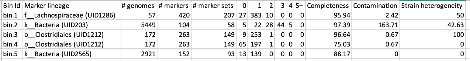
Figure 2. Example output of CheckM
Before we can visualize and plot the tree we will need to convert the reference ID names used by CheckM to taxon names. We have already prepared a mapping file for renaming the tree (rename_list.tab). We can then do this easily with the newick utilities (http://cegg.unige.ch/newick_utils).
To do this, run the following command:
cd /opt/data/
nw_rename checkm_answers/concatenated.tre assemblies/rename_list.tab > renamed.tree
Visualising the phylogenetic tree
We will now plot and visualize the tree we have produced. A quick and user- friendly way to do this is to use the web-based interactive Tree of Life (iTOL): http://itol.embl.de/index.shtml
iTOL only takes in newick formatted trees, so we need to quickly reformat the tree with FigTree (http://tree.bio.ed.ac.uk/software/figtree/).
In order to open FigTree, open a new terminal window (without docker) and type figtree
Open the renamed.tree file with FigTree (File -> Open) (file is in /home/training/Binning) and then
select from the toolbar File -> Export Trees. In the Tree file
format select Newick and export the file as renamed.nwk (or choose a name you will recognise if you plan to use the shared account described below).
To use iTOL you will need a user account. For the
purpose of this tutorial we have already created one for you with an
example tree. The login is as follows:
User: EBI_training
Password: EBI_training
After you login, just click on My Trees in the toolbar at the top and select
IBD_checkm.nwk from the Imported trees workspace.
Alternatively, if you want to create your own account and plot the tree yourself follow these steps:
1) After you have created and logged in to your account go to My Trees
2) From there select Upload tree files and upload the tree you exported from FigTree
3) Once uploaded, click the tree name to visualize the plot
4) To colour the clades and the outside circle according to the phylum of each strain, drag and drop the files iTOL_clades.txt and iTOL_ocircles.txt present in /home/training/Data/Binning/iTOL_Files/ into the browser window
Once that is done, all the reference genomes used by CheckM will be coloured according to their phylum name, while all the other ones left blank correspond to the target genomes we placed in the tree. Highlighting each tip of the phylogeny will let you see the whole taxon/sample name. Feel free to play around with the plot.
Does the CheckM taxonomic classification make sense? What about the unknowns? What is their most likely taxon?